
TrafficViewer Pro Software Manual
Last Updated 8/23/2013
Table of Contents
1.3 Installing TrafficViewer Pro.
2.0 The TrafficViewer Pro Desktop.
2.1.2 The Communications Menu.
2.2 The TrafficViewer Pro window action buttons.
2.3 The TrafficViewer Pro status bar.
2.4 The Communications panel action buttons.
7.0 Managing Classification Rules and Schemes.
7.1 The Classification Rules Panel.
7.2 Overview of raw data processing in TrafficViewer Pro.
7.4.1 The Classifications Tab.
7.4.2 The Classification Rules Tab.
7.4.3 The Unclassified Handling Tab.
This manual is available in full color PDF format at this manual download.
This manual describes the TrafficViewer Pro software which fully supports VehicleCounts.com counters (such as the PicoCount 2500, and the PicoCount 4500). When a counter is connected to TrafficViewer Pro through the download cable, the counter is automatically detected and the appropriate screens for the counter will appear. You may download a fully functional copy of the TrafficViewer Pro software at any time from trafficviewerpro.vehiclecounts.com. Once installed, it can be set up to auto-update periodically to more recent versions when you are connected to the Internet. In addition to updating itself, the TrafficViewer Pro can also update the internal programs (firmware) of any counters attached to TrafficViewer Pro if, and when, new firmware releases are made for the counters.
The TrafficViewer Pro was designed to be as simple as possible for the user, hiding little used, confusing, or advanced features in "Advanced" or "Preferences" sections of the program.
There is also the TrafficViewer Pro Beta* software, which is the pre-release version of the TrafficViewer Pro software. The Beta* version is 100% compatible with the release version, it may have some new features or fixes that are not in the release version. If you like the latest versions of software at all times, you may wish to use the Beta* version, however, be warned that it has not been tested as thoroughly as the release version. You may download a fully functional copy of the TrafficViewer Pro Beta software at any time from beta.vehiclecounts.com.
This manual covers both versions of the software.
This manual is written with the assumption that you are familiar with automated traffic counters, their setup and usage. It also assumes you are familiar with the terminology used in the traffic counting industry. That being said, here is a glossary of many of the terms used in this manual:
Anchor. The device used to secure the air hose to the roadway or shoulder.
Dwell. The time after a hose is “hit” before another “hit” will be recorded. Also known as deadtime, recovery time, response time, delay after hit time, etc. In the case of timestamp recording machines like the PicoCount, the dwell time can be adjusted after the data is collected to aid in cleaning up the collected data. In these machines there is also a minimum settable dwell time which is the built in hardware delay time that all timestamp data is collected with.
Grip. The device used to attach the hose to the anchor.
Hit. When a moving vehicle tire strikes a hose generating an air pulse.
Hose. Specifically, the rubber air hose (pneumatic hose) used for traffic sensing.
Multiple-Study. Several traffic studies done without downloading the data between studies.
Occupancy. In multi-lane roadways, it is the total of vehicles in each lane.
Roadway. The active surface of the highway, road, or driveway that vehicles travel on.
Study. The setup and collection of roadway data in one session. In other words, if you reset the PicoCount counter, set it up on a roadway, collect the data, then download the data, you have completed a study. If you set the counter up and collect data more than one time before downloading the data, then you have collected multiple studies.
Timestamp. A data storage method where every event (such as a hose hit) is recorded as a time count.
Traffic Study. In our case, it is the data gathered for a period of time. There are a variety of other terms used in the industry for the same thing, such as "Session", "Counts", or just "Study".
The following trademarks are used throughout this manual:
Windows® is a registered trademark of Microsoft Corporation.
PicoCount is a trademark of R&R Technologies, Inc.
TrafficViewer Pro is a trademark of R&R Technologies, Inc.
VehicleCounts.com is a trademark of R&R Technologies, Inc.
If you have not installed TrafficViewer Pro yet, go to trafficviewerpro.vehiclecounts.com. and download the latest TrafficViewer Pro installer. Once you have downloaded the software, start it. The total installatiion takes less than a minute. The installation does not leave a shortcut on your Windows desktop, instead you will find the software in the Windows “Start” menu. You can create your own shortcut to your desktop from there.
TrafficViewer Pro communicates with the counters via serial ports. In almost all computers today, the serial port is generated with a USB to serial cable. VehicleCounts.com offers a USB download cable for this purpose. If you are using the USB download cable, the first thing you will need to do is install drivers for it. The USB driver install program may be downloaded from our website at www.vehiclecounts.com/downloads.html.
To determine if you will need to install drivers, plug the download cable into your PC. You will see a Windows info screen pop up saying "New hardware found".
If you are lucky, Windows will recognize the USB download cable and automatically install/activate the drivers and you will see a Windows info screen pop up saying "Hardware installed and ready to use". If this is the case, you are ready to go.
If Windows does not recognize the USB device or the appropriate drivers, the driver install wizard should pop up. Close the wizard. Then download and run the Driver Install program from our website. Once the installation is complete, the USB download cable should properly connect each time you plug it in.
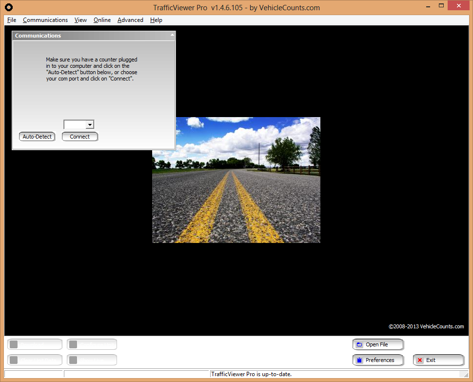
When you start TrafficViewer Pro, it will open up with its desktop view which should look something like:
The TrafficViewer Pro desktop view consists of a standard Windows® title bar, a standard Windows® pull-down menus bar, task specific panels (like the Communications panel showing above), the Action Buttons bar (across the bottom), and a standard Windows® status bar at the very bottom of the desktop view. In the above view, the TrafficViewer Pro is waiting for you to connect to a counter, or to open an existing data file. Note that the four action buttons in the lower left corner of the desktop are greyed out, they only become active when a counter product is connected.
So lets get started understanding the menus and options for the TrafficViewer Pro software:
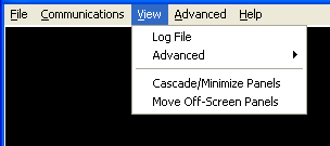
Across the top of desktop is a conventional windows pull-down menu bar showing 6 menus:
![]()
You may find some menu items that are greyed out (or dimmed), which means they are not active or available. Menu items automatically become active when the software is in a task where the menu item would be appropriate. In this section we describe each of the menu items.
Note! The file menu items Save, Export Data, and Print Reports will be grayed out when there is no data file opened (or downloaded).
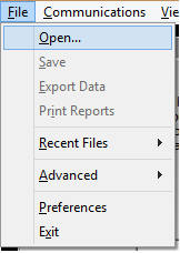
Open... Allows you to open an existing data file. To activate it, highlight Open... with your mouse and left-click on it. The menu item is also available as an action button at the bottom right of the TrafficViewer Pro window. An Open File window will appear. This window will be pointing to the default data directory (set in preferences - see below), or to the last directory you opened or saved files to in TrafficViewer Pro:
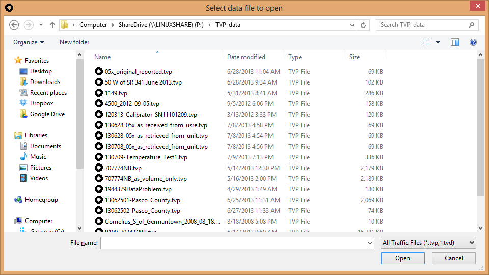
You may browse to your desired file in this window. Once you have found the file, highlight and double-click on it to open the file.
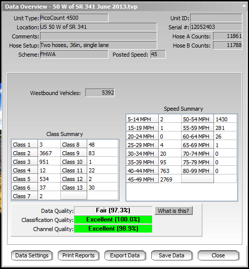
If you selected a data file that TrafficViewer Pro recognizes, you will then see a Data Overview screen pop up similar to the one below. See the Data Overview Window section below for detailed descriptions of this window.
Save. Allows you to save an open data file. To activate it, highlight Save with your mouse and left-click on it. This menu item is also available as a Save Data button on the Data Overview panel. A Save Data As... window will appear. This window will be pointing to the default data directory (set in preferences - see below), or to the last directory you opened or saved files to in TrafficViewer Pro:
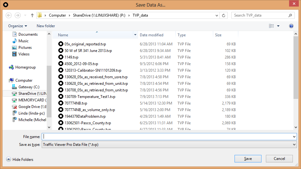
Type in the filename you would like the file to have. You do not need to type the ".tvp" extension; that will automatically be tacked on when you save the file.
Export Data. This item allows you to export an open data file into an industry standard data format such as *.CSV, *.PDF, or a variety of *.PRN types. Note that the *.CSV is a type of file which can be read by most spreadsheet (such as Excel) and database programs. To activate it, highlight Export Data with your mouse and left-click on it. This menu item is also available as a button on the Data Overview panel. If you are doing a speed/classify export, the following window will appear:

The settings in this window are detailed below in the Exports section.
Print Reports. This item allows you to create printed reports from an open data file. To activate it, highlight Print Reports with your mouse and left-click on it. This menu item is also available as a button on the Data Overview panel. If you are doing a speed/classify report, the following window will appear:

The settings in this window are detailed below in the Reports section.
Recent Files. This menu item will pop up a list of the last 10 data files which you saved or opened.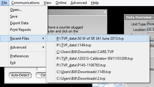
This can be useful for quickly re-opening a file that you had opened recently.
Advanced. This menu item allows you to save current data in a format that older versions of TrafficViewer Pro can read. Beginning with version 1.4.x.x, the data in the saved raw data files is stored in a newer format that the older versions of TrafficViewer Pro cannot properly process.
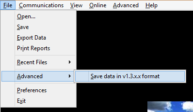
Clicking on this menu item will cause the following window to pop up:
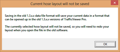
Clicking on OK will open up a save dialog like this:
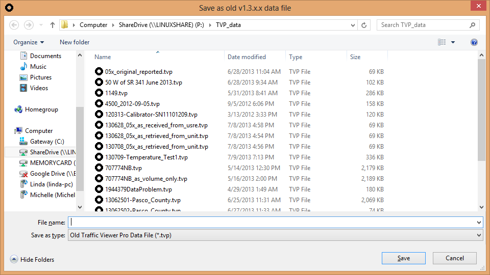
Type in the filename to save the data as and click on Save. Finally a small window will pop up like:
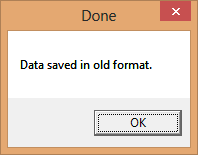
Just click on OK and your are done.
Preferences. This menu item opens up a Preferences window which will allow you to view and change various TrafficViewer Pro preferences (settings). To activate, highlight the Preferences menu item and click on it. This menu item is also available as an action button in the lower right of the TrafficViewer Pro desktop window.
See the Preferences section below for detailed descriptions of the tabs and settings.
Exit. Clicking on this menu item will close the TrafficViewer Pro program. This menu item is also available as an action button in the lower right of the TrafficViewer Pro window.
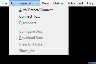
This screen shows the communications menu when a PicoCount is not connected. Note how the items that are not appropriate are greyed out.
Auto-Detect/Connect. Clicking on this menu item will cause the TrafficViewer Pro to scan all the active windows serial ports, looking for a PicoCount unit. This menu item is also available as an action button in the Communications window. See the Communications section below for more details.
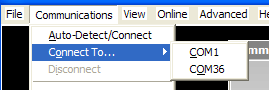
Connect To.... Clicking on this menu item will pop up a list of the available Windows serial ports. Highlight and click on the serial port the counter is attached to. This menu item is also available as an action button in the Communications window. See the Communications section below for more details.
Disconnect. Clicking on this item will disconnect from a connected unit. A similar action can be accomplished by simply unplugging the counter. This menu item is also available as an action button in the Communications window. See the Communications section below for more details.
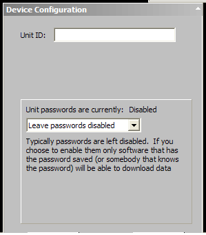
Configure Unit. Clicking on this menu item will pop a up a window which will allow you to assign the unit ID and allow you to enable/disable password security. This menu item is also available as an action button at the lower left side of the TrafficViewer Pro window.
Download Data. Clicking on this menu item will begin a data download from a connected counter unit. This menu item is also available as an action button at the lower left side of the TrafficViewer Pro window. See the Downloading Data section below for more detailed information.
Clear Unit Data. Clicking on this menu item will allow you to clear the data in the PicoCount. This menu item is also available as an action button at the lower left side of the TrafficViewer Pro window.
Show Live. Clicking on this menu item will pop a up a window which shows axle hits in real-time. This menu item is also available as an action button at the lower left side of the TrafficViewer Pro window.
Advanced. Clicking on this item will pop up the Activation Code item. This would be used for establishing or resetting passwords, or for extending the days of activity in demo units, or for converting demo units to fully active units.
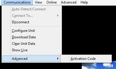
Clicking on Activation Code will pop up the following dialog:
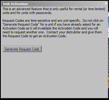
This feature is detailed below in the Unit Activation section.
Log File. Clicking on this menu item will pop up a scrollable operations log of all tasks that have been executed by the TrafficViewer Pro software.
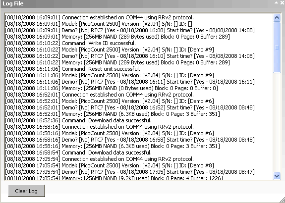
This window is useful for isolating the nature of a problem. It usually would only be used while troubleshooting. A detailed description of the log file contents can be found below in Log File Structure.
Advanced. Clicking on this menu item will activate an Additional Details window. See the Advanced View Panel section below for a detailed description of this feature.
Cascade/Minimize Panels. Clicking on this menu item will shrink all open panels on the TrafficViewer Pro window to their minimum size and stack them in a row. This would mostly be used if the window was getting too cluttered with open panels, but you still wanted them open.
Move Off-Screen Panels. Clicking on this menu item will allow you to move panels that are open, but not showing in the TrafficViewer Pro window, to a more visible location. This would usually only be needed if the TrafficViewer Pro window was re-sized with panels open.
This menu is only active when you are connected to the internet.
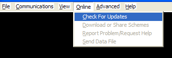
Check for Updates. Clicking on this menu item will go online to see if your current TrafficViewer Pro is the latest version. If so, you will be asked if you wish to update the software. This will only work if you are connected to the internet.
Download or Share Schemes. You would click on this item if you wished to receive or share a Classification scheme with another user. (If greyed out, this feature is not yet implemented).
Report Problem/Request Help. Click on this menu item if you wish to report a problem, or request help online. (If greyed out, this feature is not yet implemented).
Send Data File. Click on this menu item if you wish to send the current open data file to VehicleCounts.com. Generally would be used for troubleshooting. (If greyed out, this feature is not yet implemented).
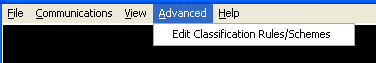
Edit Classification Rules/Schemes. Clicking on this menu item will put you into a window that will allow you to edit and manage the classification schemes that the TrafficViewer Pro uses for processing data. See the Classification Rules and Schemes section below for more details.
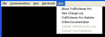
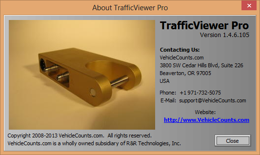
About TrafficViewer Pro. Clicking on this menu item will pop up an information screen about the software, version number, copyright notices, etc.
View Change Log. Clicking on this menu item will display a list of all the changes made to each released version of the TrafficViewer Pro software.
TrafficViewer Pro Website. Clicking on this menu item will connect you to the TrafficViewer Pro website using your operating or default browser -- assuming you are connected to the internet at the time you click on this item.
Online Documentation. Clicking on this menu item will open up this documentation in your web browser.
Contact VehicleCounts.com Clicking on this menu item will pop up a help request form, which will be automatically sent to VehicleCounts.com if you are connected to the internet. (If greyed out, this feature is not yet implemented).
Contact your Distributor. Clicking on this menu item will pop up a help request form, which will be automatically sent to the distributor you select, if you are connected to the internet. (If greyed out, this feature is not yet implemented).
There are action buttons sprinkled across the bottom of the TrafficViewer Pro window. If a button is greyed out (or dimmed), that action is not currently available. Most of the action buttons can also be accessed from the Menu items discussed above.
![]()
Download. Clicking on this button will begin a data download from a connected counter unit. See the Downloading data section below for more detailed information.
Clear Unit Data. Clicking on this button will issue a clear data command to an attached counter. However, you will first be prompted to save any unsaved data.
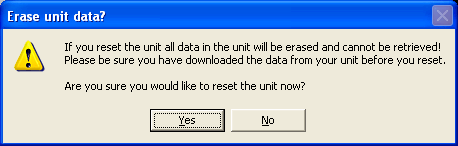
If you choose yes, the data in the unit will be erased and the real-time clock in the unit will be synchronized to the real-time clock of your PC.
Configure Unit. Clicking on this button will open the device configuration window.
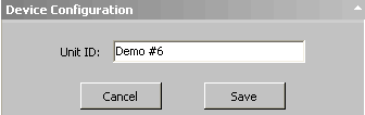
Currently the user can only configure the Unit ID. The Unit ID besides displaying in status windows, will also appear in all reports, and as part of the export file header.
Show Live. Clicking on this button activates a live data view window.
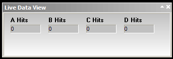
Upon entering this window, the counters will be zero'd. Each time an A, B, C, or D hose hit is recorded, the appropiate counter will bump. This would be useful in the field to verify your hose connections if you have a laptop or PDA available to monitor the connection.
Open File. Clicking on this button will pop up a standard open file window. You would use this button to open an existing data file. For instance, you may choose to download and store a series of studies, leaving the report generation to a later time, so you can get the counters back out into the field in the quickest time.
Preferences. Clicking on this button opens the preferences window. See the preferences section detailed below.
Exit. Clicking on this button exits the TrafficViewer Pro software.
At the very bottom of the TrafficViewer Pro window is a status bar which shows the current communications status.
![]()
The first field shows the com port status (opened or closed). The second field shows the PicoCount connection status. This is discussed in more detail in the Communications section below.
These buttons are also available as items in the Communications pull-down menus. This window is discussed here, because it is always present when TrafficViewer Pro is running. All of the other sub-windows of TrafficViewer Pro come and go depending on what you are doing, but the Communications window always stays on the TrafficViewer Pro desktop (it can be minimized when you are not needing it).
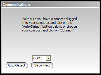
Auto-Detect. Clicking on this button will cause the TrafficViewer Pro to scan all the active windows serial ports, looking for a counter. See the Communications section below for more details.
Connect. Clicking on this button connects to the com port highlighted in the pull-down list directly above the connect button. The pull-down list will have all available Windows serial ports listed. See the Communications section for more details.
This section describes the Communications features of the TrafficViewer Pro and its various options. TrafficViewer Pro communicates with a variety of counters via the standard PC serial ports and USB virtual serial ports. The data frame for all communications consists of 1 start bit, 8 data bits, 1 stop bit, and no parity. The communication data rate will depend on the counter product interfaced to TrafficViewer Pro. Once TrafficViewer Pro detects the type of counter connected, it sets the appropriate data rate (also called Baud rate). For our counters, the normal Baud rate is 115,200 Baud, however during downloads TrafficViewer Pro will automatically raise the Baud rate to the maximum allowed on the installed serial port.
On first starting up TrafficViewer Pro you will see the following TrafficViewer Pro desktop:
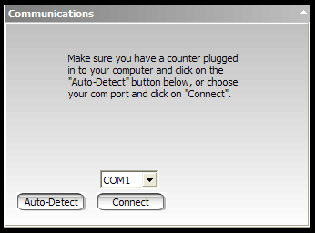
The Communications panel begins as shown above, waiting for you to take some action. Note that the action buttons in the Communications panel are also available via the standard Windows® pull-down menu “Communications”.
Once a counter is connected to the download cable, you can begin communications with the counter by clicking on the Auto-Detect or the Connect button. If you are using a USB download cable, it must be plugged into the computer before starting TrafficViewer Pro software, otherwise it will not be detected. If you connect the cable to the PC after TrafficViewer Pro software is already running, simply close the software and restart it.
Most users use the Auto-Detect button. In this case, TrafficViewer Pro will scan all active and available (not already opened) Windows® serial ports, sending detect commands to each serial port in sequence until it detects a recognized counter.
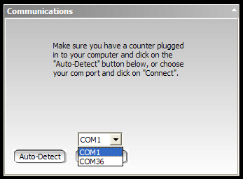
Some users will "know" the serial port number that the counter is attached to and may prefer to connect directly by first highlighting the com port on the pull-down list just above the connect button, then clicking on Connect. In this case, TrafficViewer Pro will send the detect commands only to the com port specified. This scheme can be useful in systems that have many serial port connections, particularly Bluetooth connections, which tend to have very long wait delays and may make the Auto-Detect rather slow.
If you use the Auto-Detect button to scan for a connection but do not have anything attached, you will notice at the very bottom left of the TrafficViewer Pro Desktop the status fields will show the connection progress. Say there are two serial ports active, COM1 and COM36. When you press the Auto-Detect button, the status field will say "COM1 Opened", followed a few seconds later by "COM36 Opened", then followed a few seconds later by "COM36 Closed". Just to the right of this message, the connection status will show "All ports scanned, no device detected."
![]()
If a counter is attached to COM36 and you click on the Auto-Detect button, the status field will say "COM1 Opened", followed a few seconds later by "COM36 Opened", then a few seconds later the connection status message "Device Info Read Successfully".
![]()
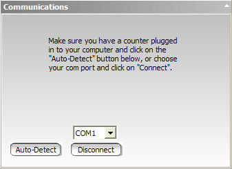
After you have finished with the counter and unplug it, the status bar at the bottom of the window will display something like this:
![]()
Notice that the button in the Communications panel that was labelled “Connect” is now labelled “Disconnect”. You may now plug the download cable into another PicoCount and it will automatically connect without you having to push any buttons.
If instead of the Auto-Detect button being pressed, you chose to select the COM36 and clicked on the Connect button, with no counter attached you would see the status field will say "COM36 Opened" and the Communications panel “Connect” button will now read “Disconnect”.
Once a device detection and connection is made by either method, when you unplug the counter, the connection state will still show "COM36 Opened" and the status message will say "Device Disconnected". (Note the original Connect button changed to Disconnect).
The communications port will stay in this state until you close TrafficViewer Pro. If you connect to a counter and leave it connected more than 5 minutes with no operations, TrafficViewer Pro will time-out the connection, close the com port, and display the status message "Operator not present - timed out". This is done to conserve battery life in the counter units.
If a PicoCount 4500 is attached to the PC via the download cable when you pressed the “Auto Detect”, or “Connect” button as described above, the Communications panel will now look something like this when connected:
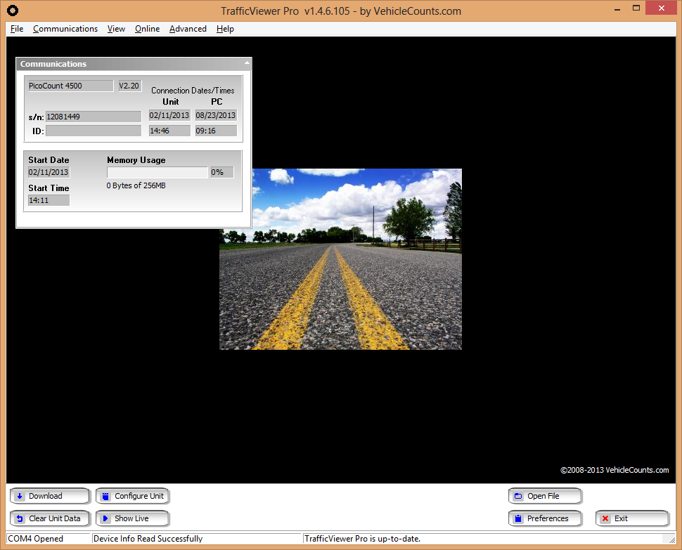
Note that the four action buttons in the lower left of the TrafficViewer Pro Desktop have become activated when a device is connected.
You are now ready to download data or configure the counter, but first, lets look at the “Connected” Communications panel in more detail.
This panel view gives you a snap-shot of some useful information and status of the connected counter. When things seem to go wrong, careful inspection of this screen may shed light on the problem.
Starting with the upper left field. This field shows what device is connected to TrafficViewer Pro which in this case is the PicoCount 4500. The field to the right is the current version of firmware (software) inside the counter. If a more recent version is available, a bright yellow panel will pop up letting you know a new version is available and offer to upgrade it now (that is assuming you have the latest version of TrafficViewer Pro installed). If you have data to download, do this first before upgrading the unit firmware. This information is also presented on all reports, exports, and saved data files.
The field below the unit type field is the unit Serial Number. This field should always be filled in with a meaningful string of numbers which are also etched into the back panel of the case. Every VehicleCounts.com counter manufactured has a unique serial number assigned to it for keeping track of repair histories, warranty, and occasionally ownership. The serial number is also presented on all reports, exports, and saved data files.
The field directly below the serial number is the unit ID field. This field is for the user to enter their own ID for the counter. It can be changed by clicking on the “Configure Unit” action button at the bottom of the TrafficViewer Pro desktop. This information is also presented on all reports, exports, and saved data files.
To the right of these two fields are four fields containing the current Date/Time in the connected counter, and the current Date/Time on your PC at time of connection. These two times should always be nearly identical. The causes of differences are time drift of the counter (usually only seconds at most), using a different PC to download the data than was used to “reset” the counter (usually only seconds or minutes). Movement of the counter across timezones, or daylight savings changes (usually hour changes).
The two fields in the lower left of the panel show the Start Date/Time of the unit. This is when the unit data was last cleared. Normally, it should be some time just before the last study was performed. Once in a while, the unit data won’t be cleared, and when data summary comes out looking unexpected, it is because there are two or more studies in the unit. These can be sorted out at report or export time, but it can be a hassle.
The final field in the lower right of the panel shows how much memory was used since the unit data was last cleared. Most studies will be a few tens of kilobytes to a few megabytes, which is only a small fraction of the total capacity of the counter memory.
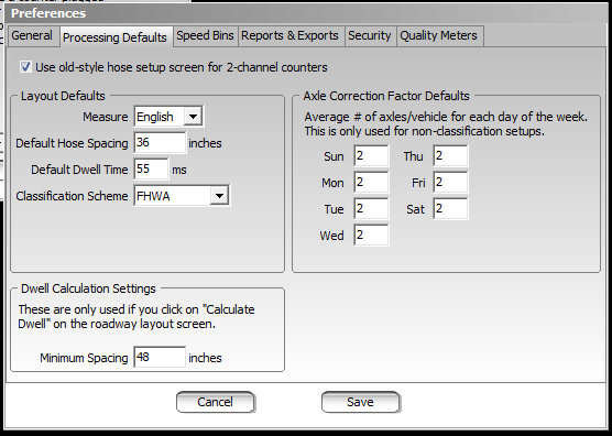
This is an “advanced” section and describes the Preferences settings for TrafficViewer Pro. The Preferences Panel allows you set a variety of parameters and default settings that will be applied to downloaded data, reports, or software updates. If the settings in this section don’t make sense, or you don’t know the significance of them, it is best not to change anything. Our factory defaults for the preferences will work for almost all situations.
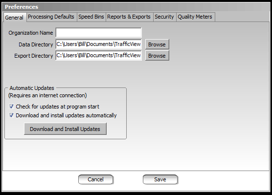
If you click on the Preferences action button or select it in the Files menu, you will get the following panel:
The preferences are separated into 6 categories indicated by the tabs, each consisting of a variety of user fields and check boxes.
Is the first tab and is presented when you first enter the preferences, and covers some general configurations for TrafficViewer Pro.
Organization Name. In this field you can enter your company or organization name which will then show up on all Reports, Exports and saved files.
Data Directory. You can type in or Browse to the folder that you wish to be the default directory for all downloaded data storage. Note, when storing downloaded data, you can change the folder at that time to another folder before storing the data, and all following data storage will be in the new folder, unless you change it again. However, when TrafficViewer Pro is closed and re-started, the data directory specified in Preferences will once again be the default data folder.
Export Directory. You can type in or Browse to the folder that you wish to be the default directory for all exported data. Note, when saving exported data, you can change the folder at that time to another folder before saving the data, and all following export data saving will be in the new folder, unless you change it again. However, when TrafficViewer Pro is closed and re-started, the export directory specified in Preferences will once again be the default export folder.
Automatic Updates. Is a box that contains a couple of checkboxes and a command button. These only work if your computer is connected to the internet. The checkboxes allow you to specify if you wish TrafficViewer Pro to check for new updates each time you start TrafficViewer Pro up. And to automatically download and install new updates if they are detected. There is also a command button that will immediately check for, download and install latest updates.
In this tab, there are a series of fields that dictate how timestamped data is to be interpreted. Note that these settings in no way affect the timestamp data that is downloaded and saved, only the interpretation of the data for data views, reports and exports. Each of these fields can be overwritten on a case by case basis during the download.
Measure. Is a field where you can select English or Metric representation of data. This field will dictate how processed data is displayed, reported and exported. If English is specified, then speeds will be in miles per hour (MPH), distances will be in inches, and dates will display as mm-dd-yyyy. If Metric is specified, then speeds will be in kilometers per hour, distances will be in centimeters, and dates will be displayed as dd-mm-yyyy.
Default Hose Spacing. Is a field where you set the default hose spacing for all downloads. When you download the data, you can change this setting on a case by case basis if needed. Most agencies use standardized spacings for all of their counters and this is what you would normally set the default to. The hose spacing is needed to accurately calculate vehicle speeds (and classes). It does not need to be set to any particular value if you are only doing volume studies.
Default Dwell Time. Is a field where you can set the minimum dwell time for hose hits. This term goes by a variety of names, like “sensor timeout”, “sensor deadtime”, “recovery time”, etc., but they are all the same. Basically, when a hose hit occurs, the hose sensor is disabled for a specified period of time before the sensor is allowed to detect another hit. This is described in detail in a later section. In earlier generation counters, this dwell time was done in hardware, but with modern timestamp counters, the hardware dwell times are kept as short as practical (as short as 10ms) and software is used to emulate longer dwell times. Choosing appropriate dwell times will depend on how you do the majority of your studies.
Classification Scheme. Is a field where you can specify the vehicle classification scheme you wish to apply to the processed data. The available schemes are on a pull-down list; the choices are FHWA, AustRoads, Swedish, and any custom schemes you may have created. If you are doing volume only counts, this field does not apply.
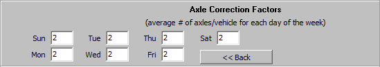
Axle Correction Factor Defaults. This box contains a field for each day of the week. These factors are applied to volume only data. Normally most data collected is cars, SUVs, and pickups, which have two axles per vehicle. When the volume of multi-axle (more than two) vehicles becomes large relative to the two axle vehicles, it can cause the volume counts to read high. Factors is a way to compensate for this issue. From historical data (or hand-count data), for instance, if you know that the actual number of vehicles times two is only 95.0% of the total axles because of a large number of multi-axle vehicles, you would get a more accurate count by using 2.105 Axles/Vehicle when processing the data. The different factors for different days of the week allow you to correct for the fact that multi-axle vehicles mostly travel on “working days”.
Dwell Calculation Settings. When you do a data download from a counter, a Data Settings screen pops up. One of the options on this page is to allow the TrafficViewer Pro software calculate the optimal “Dwell Time” for the data. That calculation uses the Posted Speed and the minimum spacing between axles you would like resolved. This section allows you to specify the minimum spacing between axles that you would like detected. This would normally be set to the minimum spacing expected in multi-axle trucks.
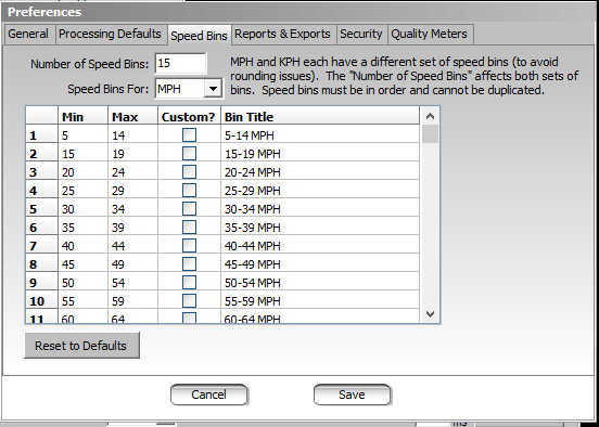
In this tab, you may set up the Speed bins you wish processed speed data to be placed into. The default is 15 bins, with the speeds shown as MPH above (there is also a default for KPH). If you wish the speeds to be categorized into more or less bins, just change the Number of Speed Bins setting. The default bin size is in 5 MPH (10 KPH) steps (except the first and lowest bins are 10 MPH and 15 KPH respectively). You can change these by checking the Custom? checkboxes for each bin you wish to change the range of. If you do this be very careful that the bins are in order and there is no overlap of speed ranges. Ranges are defined from xx.000 to yy.999 (i.e. 15-19MPH is 15.000-19.999MPH).

This tab allows you to specify the reports and exports default settings.
Bin Interval. Is the interval in minutes that all reports and most exports total counts. The most common interval is 60 minutes (1 hour). In the case of the example above, at report generation time, vehicle counts and totals for each 15 minutes of time during the study would be displayed. Shorter interval times make the reports longer and for large files make the computation time noticably longer. The shorter times are mostly used during traffic analysis, to figure out the affects on traffic flow of signal lights, etc. You can specify data in 1,2,3,4,5,6,10,15,20,30, and 60 minute intervals.
Export Type. Is the default export you would normally use if you were exporting data. TrafficViewer Pro supports a variety of export types, including several PRN type exports (many states have their own variance of the federal standard). The currently supported exports are: CSV,Standard; PDF; PRN, Standard (federal); PRN, ConnDOT (Connecticut); PRN, FDOT (Florida); PRN, HDOT (Hawaii); PRN, INDOT (Indiana); PRN, NYSDOT (New York State); and PRN WSDOT (Wisconsin). This list is constantly being expanded.
PRN Exports. This box contains default settings for PRN exports. There is a checkbox to automatically create a new file for each day’s data in a multi-day study. You can set a default naming convention for the files, and you can have some custom text added to each file.
Timestamp Exports. This box allows you to specify the format of the timestamps. Currently you may specify “seconds since start date/time”, “Days since December 30,1899”, or “Readable date/time”. The seconds or days formats are for programs that will be using the data for computations. The readable data/time is for end users that will be visually inspecting the data. Note that at the time you do the export, you can change your selection to any of the other settings for that particular export.
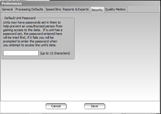
The PicoCount counters have built-in password security that by default is not activated. If a PicoCount with its password activated is connected, this default password is first tried on the unit, if it fails, then the unit will ask the user for his/her password. This is most convenient for daily use on a known “controlled” computer so that the operator does not have to enter passwords for each and every counter he connects to.
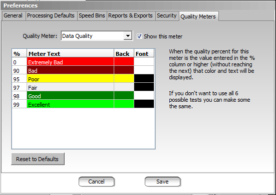
The TrafficViewer Pro software displays three “Quality Meters” in the Data Summary screen. This panel lets you customize the test percentages and look (color) of the meter. You can also choose to not show the meter(s). The Quality Meter field is a pull-down list of the three meters: Data Quality, Classification Quality, and Channel Quality. These meters are discussed in a later section of this manual.
This section covers the actions and options involved in downloading data from the counter. Once communications is established with a counter, you can download its data by clicking on the action button Download, located in the lower left of the TrafficViewer Pro desktop, which should now be active. Alternatively, you can choose the Download Data menu item in the Communications pull-down menu.
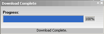
Once you click on Download, a progress panel will pop up showing the progression of the download. For short data files you may only see the Download Completed panel.
As soon as the download is complete a Data Setup panel will pop-up.
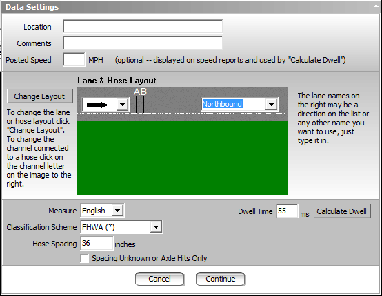
You can now, optionally, enter data into the fields Location, Comments, and Posted Speed. These fields if filled in will be stored with the raw data file and be printed in the header portion of reports and exports.
The fields Measure, Classification Scheme, Hose Spacing, and Dwell Time will be set to the values specified in the Preferences panel -- discussed earlier in this manual -- on first entry. If you change any of these values, without closing TrafficViewer Pro, it will use the new settings for all subsequent downloads. Keep in mind, the Preferences settings are your normal expected settings, but sometimes you may run a set of counts that need these fields changed.
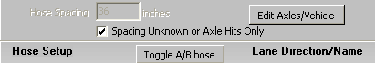
The checkbox Spacing Unknown or Axle Hits Only would normally be checked only when doing volume counts only. By checking this box, TrafficViewer Pro makes no attempt to compute speeds or classifications of vehicles. Occasionally it is useful when, in the midst of a study that is doing speed and/or classification, a hose breaks loose. This will at least allow you to get volume reports from the data. Notice that when you click on this checkbox that an Edit Axles/Vehicle button appears to the right.
Clicking on the Edit Axles/Vehicle button allows you to enter the "axles per vehicle" (nominally 2.00) for each day of the week. If you know the statistical "mix" of vehicle types for your area and wish the counts to more accurately reflect the number of vehicles you can apply the Axles/Vehicle factor to the data. For instance, if you know that the actual number of vehicles times two is only 95.0% of the total axles because of a large number of multi-axle vehicles, you would get a more accurate count by using 2.105 Axles/Vehicle when processing the data.
In the Lane and Hose Layout section of this panel, if the hose layout you used is not displayed (two hoses across a single lane is showing in this example), then click on the Change Layout button.
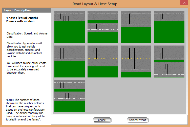
Since this was a PC4500 four channel counter, you will see all the layout options available. If it had been a PC2500 two channel counter this same screen would look like:
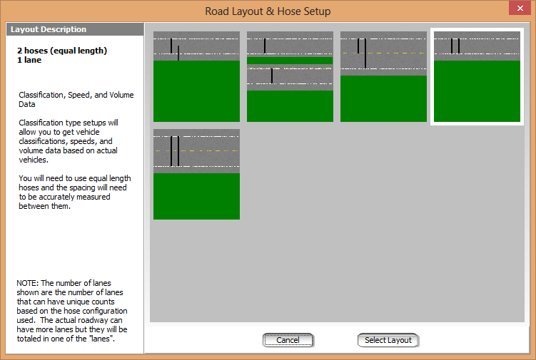
Highlight the layout that best represents how the counter was connected and click on the Select Layout button.
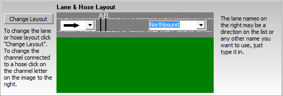
In this example we have chosen the two hoses across a single lane layout which is the most common configuration for speed and classification studies in a single lane. In the graphic, there are three fields you can set, first thing you would do is select the lane direction from the pull-down list. Then you specify which way the cars were going in the lane by selecting the approriate arrow, then you specify which hose gets hit first. In this layout, we have chosen Northbound for the lane travel direction, traffic moving from left to right, and the A hose would be hit first. If the B hose was being hit first, then place your cursor over the hoses in the graphic and you can click on them to swap the A and B hoses, so that B hose will be hit first.
Once the panel represents your study data correctly, you may click on the Continue button. If you are not sure of all the correct settings, you can continue on anyway, and come back to this screen later from the Data Overview panel -- even after saving the data.
Note! If you installed TrafficViewer Pro over version 1.3.x.x or earlier, by default, it will display the older version Data Settings window for PC2500 counters. This is to help ease the user into the newer way of doing things. There is a checkbox in the Preferences, Processing Defaults tab that may be unchecked to get the new screens described above.
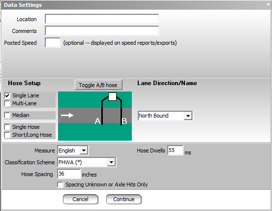
check the appropriate checkbox that best represents your hose setup in the field. As you check the checkbox, you will notice the graphic to the right of the checkbox will change. This gives you a pictorial representation of your hose setup.
For speed and classification studies, the first two checkboxes Single Lane, or Multi-Lane, would be appropriate. When either of these boxes is checked you will notice that the graphic shows two parallel hoses A and B. The pictorial also shows a traffic flow arrow in one lane, if the indicated A and B hoses are backwards, then you can click on the Toggle A/B hose button above the graphic to reverse the hoses. Most of the time you would set out the hoses with the A hose being struck first, but sometimes, the person laying out the hose may reverse the hoses.
For volume only studies, you would normally select one the the last three checkboxes Median, Single Hose, or Short/Long Hose. Occasionally, for studies only needing a single hose, you may opt to set down two parallel hoses to improve to chances of a successful count (in case one hose breaks free, etc.), which in this case, you would check the Single Lane checkbox and the Spacing Unknown or Axle Hits Only checkbox. Note that the Edit Axles/Vehicle button, discussed above, also pops up on the panel if one of these options is chosen.
To the right of the graphic representation of the hoses are the Lane Direction/Name pull-down list(s) for each lane. These settings will be used in your reports and exports.
Note! Any changes you make to the settings in this panel have a temporary memory and will be used for any following downloads as long as TrafficViewer Pro is not closed.
This section describes the Data Overview Panel and its various options. This panel will give you a quick overview of the collected data. In this panel you can save the data, print reports, export the data and go back and edit the Data Setup panel. You get to this panel at the end of a successful download or if you open an existing saved file.
The panel is sectioned into three major sections: The top section shows useful file information, the middle section shows a summary of the study data and the bottom section is the panel action buttons. Depending on whether you are doing volume only or speed/class studies, the middle panel can have a significant difference in appearance. An example of both follows:
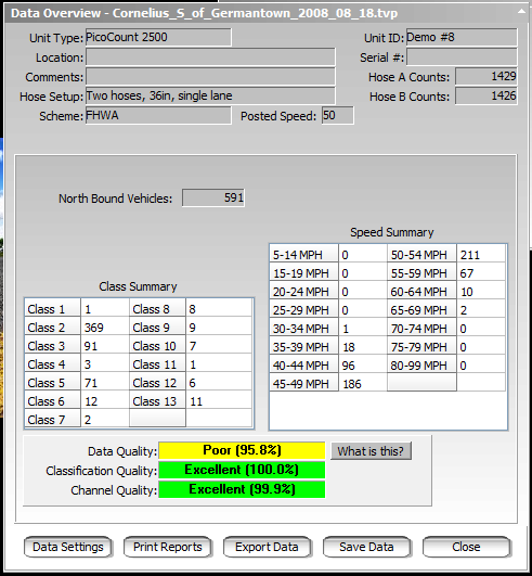
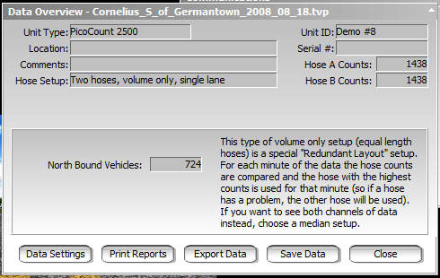
In the case of the speed/classification study, the overview shows a summary of all the data collected in the study. There are also three Data Quality meters which will give you an approximation of the expected quality of the data based on several factors such as missing, extra axle hits, how many hits were used by classification schemes, etc. These meters are a guide only and do not necessarily represent the accuracy of the collected data. If multiple studies are done on the counter without clearing it between studies, the screen represents all of the data, and if the studies had different hose layouts, the meters could become quite meaningless.
It is highly recommended that after a successful download, and before printing any reports, that you save the raw data. It is easy to do, and if for any reason you must revisit the data in the future, it will be available. It often happens that after you supply the reports to the client, they come back wanting different reports from the same data. You save the data by clicking on the Save Data action button. A standard Windows® Save File dialog will pop-up pointing to your default data folder (set in the Preferences panel, see above). If you decide to save the data in a different folder which you can do in the Save File dialog, TrafficViewer Pro will temporarily remember the new folder, for all subsequent saves. When TrafficViewer Pro is closed and reopened, the default folder will once again be used.
If the Header information (at the top of the panel) is incomplete, or the data summary indicates a wrong data setting, you can click on the Data Settings button to send you to the Data Setup panel discussed above. You can make the appropriate changes in the Data Settings panel, then click on the Continue button to return to the Data Overview panel. If you choose to change the Data Settings information, you should re-save the data with the Save Data button, so the latest settings are stored with the data.
At his point you may either Print reports of the data, or Export your data into a data format suitable for importing into a database or Excel-like spreadsheet (.csv file). These options are described in the following sections.
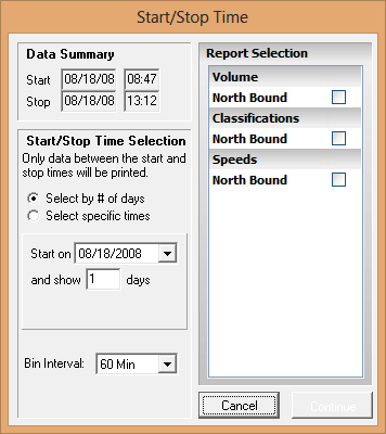
This section describes the Reports setup panels and the various reports and options available. To create a report click on the Print Reports button in the Data Overview panel.
If you are doing a speed/classify report, the following window (on the left) will appear:
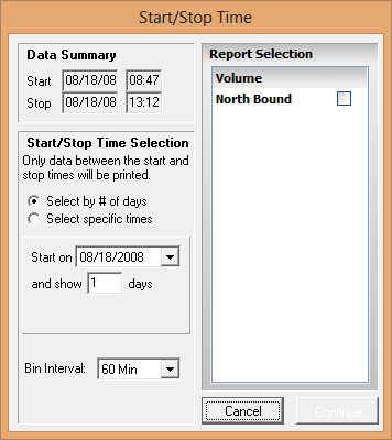
If you are doing a volume only report, a window like the one on the right will appear.
Under Data Summary, TrafficViewer Pro attempts to determine the valid data date/time range based on the recorded hits.
Under Start/Stop Time Selection you can specify the range of data to use in your report(s). You can select the data in two ways, either by whole days, or you can specify the actual date/time start and date/time stop of data to use.
If you choose Select by # of days, you can choose a starting date from the Start on pull-down list and enter the number of days of data to show in the report in the and show -- days field. With this selection, all reports start at midnight of the first day and end at midnight of the last day.
If you choose Select specific times, the fields Start and Stop will appear in the window so you can enter, start date and start time, stop date and stop time.
There is also a Bin Interval pull-down list which allows you to specify the interval of time the data will be totalized per period. In other words the bin interval of 60 minutes yields a report with hourly totals. This is the most common setting, however, if the data is being analyzed for signal light timing and other types of studies, shorter intervals may be specified. Of course, the reports could get rather large, so you have to be careful.
Once you have the report time range specified, you can select the reports you wish generated from the checkboxes on the right side of the Start/Stop Time window. Once those have been checked, click on Continue to proceed to the Print Preview window.
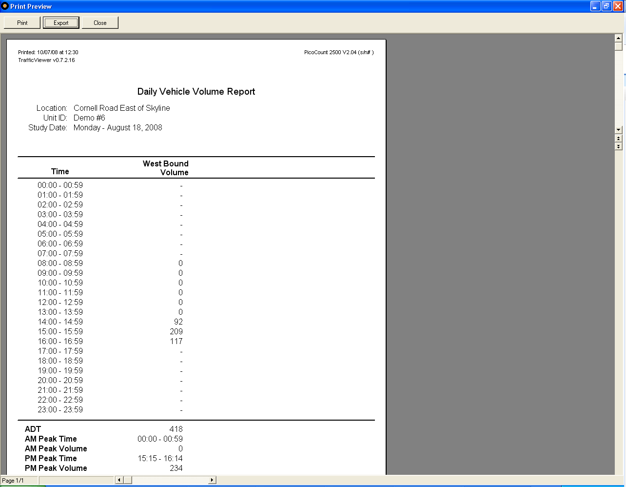
At this point, you can proceed to Print out the report or just Close the window to go back to the Data Overview panel. If you click on Print, a standard Windows® print dialog will appear where you can select the printer you wish the report printed on and proceed to printing.
This section describes the Exports setup panels and the various options available. To create an export click on the Export Data button in the Data Overview panel. If you are doing a speed/classify export, the following window will appear:
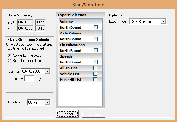
If you are doing a volume only export, the Classes, Speeds, and All-In-One checkboxes will not be present, but all the rest will.
Under Data Summary, TrafficViewer Pro attempts to determine the valid data date/time range based on the recorded hits.
Under Start/Stop Time Selection you can specify the range of data to use in your export(s). You can select the data in two ways, either by whole days, or you can specify the actual date/time start and date/time stop of data to use.
If you choose Select by # of days, you can choose a starting date from the Start on pull-down list and enter the number of days of data to show in the export, in the and show -- days field.
If you choose Select specific times, the fields Start and Stop will appear in the window so you can enter, start date and start time, stop date and stop time.
Once you have the export time range specified, you can select the exports you wish generated from the checkboxes on the right side of the Start/Stop Time window.
Finally, select the Export Type from the pull-down list. There is a standard *.csv type for exporting to a file compatible with most spreadsheets and databases. There is a *.pdf type which generates a format similar to a printout. There are a series of *.PRN types which will generate data in a format required by many government agencies, with a variety of state variations.
Once everything is selected, click on Continue to proceed to a standard Windows® Save File dialog, where you can specify the folder and filename(s) to store the export under.
This section describes the Advanced View panels and the various options available. These panels can give you much more insight into how data is handled and to troubleshoot faulty data. As of this writing, this option is only available for the two channel counters, only the first two of the four channel counters will show.
You select the Advance View by using the View pull-down menu, highlighting the Advanced menu item, then clicking on Show Additional Details.
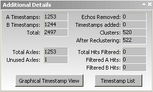
This panel shows some additional statistics concerning the data collected, and on the bottom of the panel are two action buttons, one will give you a graphical representation of the data and the other will give you a readable list of the data points.
Clicking on the Timestamp Graph will pop up the following panel:
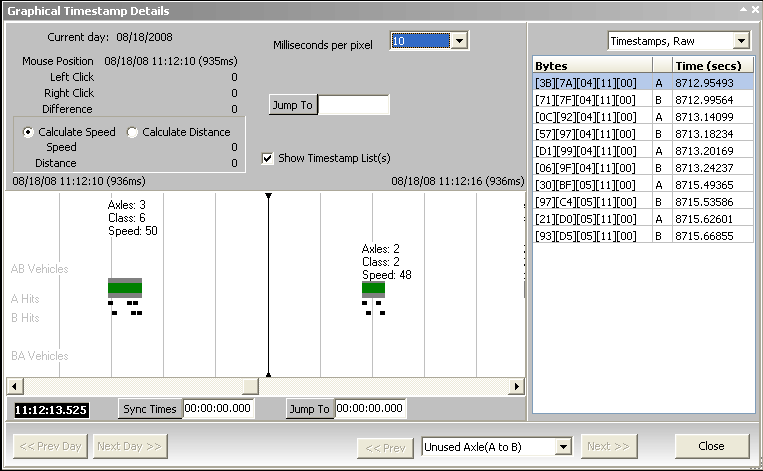
This is a very complex panel with many details. You just need to play around with it to get the hang of how everything works. This is a brief description of the panel features.
The central white area is the graphical representation of the A and B hose hits. In this area the hose hits are represented by black dots if the data point is being used or red dots if the data point is not being used (has been filtered out). The Green bar above the hose hit dots spans all of the dots used in defining a vehicle. Above these bars are details of the vehicle classification and speed. You can zoom in and out by selecting the Milliseconds per pixel pull-down list in the upper right of the panel. Once you have selected the Milliseconds per pixel, if you have a scroll wheel on your mouse, it will take over zooming in and out. The white graphical area will display one day of data at a time, the day being shown is indicated in the upper left of the panel by Current day. If the study goes over 1 day in length, the >>Prev Day and Next Day >> buttons at the bottom of the panel will activate appropriately.
Just below the graphical data scroll bar is a time box in black which indicates the time in (hh:mm:ss.mmm) at the center line of the white area.
To the right of this is a field called Sync Times which is very useful for synchronizing the timestamps to a video of the same traffic. This is done by positioning the vehicle being used for synchronization on the center line of the graphical display, then advancing the video until the same vehicle is centered in the video display. At this point you enter the video display time into the sync times field, then click on the Sync Times button. Now the time box in black will reflect the time on the video tape as you pan around the data.
To the right of the white area there is a list of the timestamps for all the axles currently showing on the graphical display. If you do not want this list, you can uncheck the checkbox directly above the list. The graphical view will then expand to fill the whole area. Also, you can view the timestamp list in several formats.
Above the white graphical area are a couple of sections that let you calculate distances between axle hits and speeds by using an A to B or B to A set of timestamps, or to calculate the time difference between any two timestamps.
To calculate time difference, position your mouse over the first timestamp dot of interest and click on the left mouse button. Next move the mouse over the timestamp dot you are trying to calculate the time difference to and click on the right mouse button. the results of the difference will show in the Difference field.
You do not have to have the mouse perfectly centered, just near the dot and it will lock onto that dot (a pop-up box will give the timestamp info about the dot when you are in the correct spot). A similar behavior will occur if you hover over the green bar representing the vehicle with your mouse, a pop-up box will give you more details about the vehicle, including axle spacings.
To calculate distances, you first need to calculate the speed of the vehicle. To calculate speed, select the Calculate Speed checkbox, then position the mouse over the leading axle A or B (dot furthest to the left) and click on it with the left mouse button. Then move to the matching A or B dot and click the left mouse button again. You will see the speed in the Speed field. Once speed has been determined, you can calculate distances. To calculate distance, select the Calculate Distance checkbox, then position the mouse over the first dot of the two you want to figure distance between. Click the left mouse button, then move to the second dot and click the right mouse button. You will now see the distance in cm or inches between the to dots in the field Distance.
This section describes how create and manage TrafficViewer Pro classification schemes. As shipped, TrafficViewer Pro has several default classification schemes, such as, FHWA and Austroads. These are industry standard schemes that follow government generated descriptions of vehicle classifications. Since counters like the PicoCount measure axle hits on pneumatic hoses, the classifications schemes have been developed on appropriate axle spacings. Normally, the default schemes are all you should need for most counting applications. However, some organizations may want a classification scheme that does not follow the default schemes, or have special schemes for special count studies.
When you click on the Advanced menu item in the main menu you will see:
Then when you click on Edit Classification Rules/Schemes you will see a panel like this:
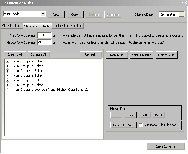
This panel will allow you to edit or create a new classification scheme. With this panel you can build up classification rules based on a variety of characteristics of the data. We will describe what each of the pieces to generating a classification scheme are and how you can go about it. Be warned, this is a section for advanced users that have a thorough knowledge of vehicle characteristics and vehicle classifications.
First though, a little information on how TrafficViewer Pro processes the raw timestamped data in a multi-pass method. The first pass through the data TrafficViewer Pro filters the data based on the hose configuration specified in the header screen. In the case of two hose setups that would allow speeds and classifications, axles in the two channels are "matched", separating forward and reverse traveling vehicles into seperate "tracks". Next, the data is scanned for the presence of air pulse "echoes" in the data and if detected, these "echoes" are filtered out. If the header indicates a "volume only" configuration, then the data requires no further processing, otherwise, the next pass would utilize the data in the Classification Scheme to attempt to classify and count vehicles.
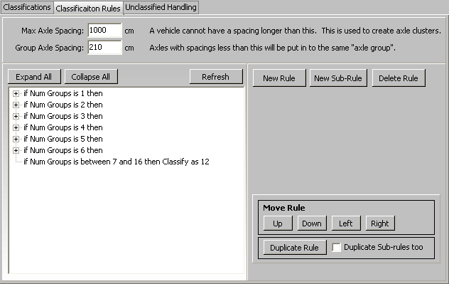
In this pass TrafficViewer Pro begins at the start of the data and generates a "cluster" of axle hits. A cluster starts with the first axle hit and continues until the Max Axle Spacing (field in the middle of the panel above) is exceeded. Note that distances can be specified in either Inches or Centimeters (You determine this in the upper right side of the panel in the Display/Enter in field).
Once the cluster is built, then the data is applied to the classification rules indicated in the large white field in the lower left side of the panel. Rules are processed sequentially from top to bottom. If all axles in a "cluster" match one of the rules, the vehicle is classified accordingly and TrafficViewer Pro then fetches the next "cluster" from the data file. If a cluster fails to process to a classification, the cluster is then is further processed according to specified options (see the Unclassified Handling tab below).
The recommended option is to re-cluster the failing cluster. A cluster is "re-clustered" by removing a pair of axle hits and running the new cluster through the classification rules. If this fails, it will continue removing single axles until the cluster is too small (less than two axles) or a successful classification has been established, at which point the removed axle hits are now re-processed until all hits in the original cluster have been resolved, or optionally discarded.
A good example of how this "re-clustering" would work would be to consider three cars "tail-gating". The original "cluster" would grab 6 axles. First pass through the rules would fail to match any 6 axle vehicle to that particular array of axle spacings, therefore, we would drop the last two axles off and re-process with 4 axles. Again, no 4 axle vehicle would classify with those axle spacings, so we would drop 1 more axle. The remaining 3 axles again fail to classify in this example, so we would drop 1 more axle. The remaining two axles would classify as a "car", so we now try processing the remaining 4 axles. Again no 4 axle vehicle would classify with the remaining axle spacing, so we drop 2 axles. When reprocessed, we would classify the two axles as a "car". Then we grab the remaining 2 axles and process them which would also classify as a "car". As a result, the original cluster would resolve as 3 cars.
Now lets analyze the Classification Rules panel in detail. The panel can be broken into three main sections, the upper part (or scheme management section), the middle part (or rules management section), and the lower part (scheme saving). Starting with the top part of the panel:
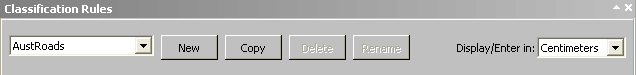
This section of the panel allows you to manage your schemes and specify how to display spacings. As shipped, TrafficViewer Pro has default schemes for FHWA and Austroads, which you will see in the pulldown list. As you add schemes, this list will grow.
New. You would click on this button if you wished to create a new scheme from scratch. When you click on it, you should see:

At this point you should Rename the new scheme to something more meaningful, but you do not have to. Note that the Delete and Rename buttons are now active. You cannot delete or rename the default schemes, that is why they were not active originally. Also note that any scheme that is not a default scheme will be followed by the (*) symbol in the list. That means that that scheme is re-nameable and deletable.
Copy. If you wish to create a new scheme from an existing scheme, you would use this button. When you click on it you will see something like this:

At this point you should Rename the new scheme to something more meaningful, but you do not have to.
Delete. To delete an unwanted scheme from the list, highlight the scheme you wish to remove in the list of schemes, then click on this button. It will prompt you to make sure that is what you really wish to do. Note that this function will only work with schemes followed by the (*) symbol.
Rename. To rename a scheme, select it on the schemes list, then click on this button to allow you to edit the name of a scheme. This function will not work with the default built-in schemes.
Display/Enter in: In this field, you select spacing information in centimeters or inches when viewing and editing the scheme rules. You can change this at any time during the viewing or editing of the scheme rules.
The middle part of the Classification Rules panel allows you to view and change the rules for the scheme highlighted in the scheme list in the upper part of the panel. This section of the panel will appear like below for the AustRoads scheme selected in the upper panel:
This panel is organized into three tabs: Classifications, Classification Rules (shown), and Unclassified Handling. We will discuss each of these tabs in order. For purposes of illustration and since we are in the USA, we will do all of the below descriptions using the FHWA scheme with measurements in inches.
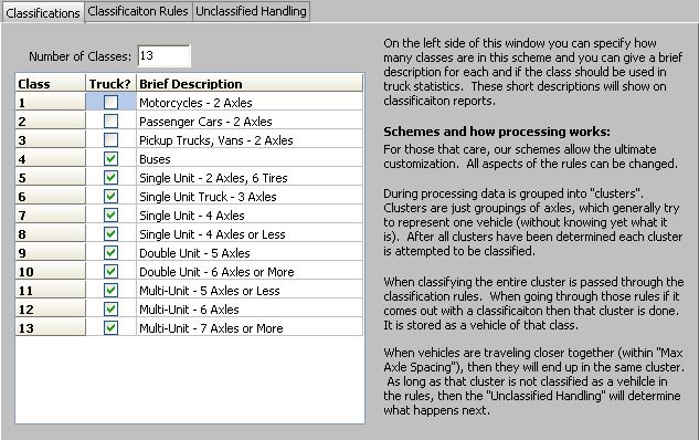
Classification schemes attempt to interpret the vehicular axle spacings into a number of "classes" of vehicles. The FHWA (Federal Highway Administration) scheme calls for 13 classes of vehicles. In the USA most federal, state and local authorities use this scheme. Some states or communities may require a slightly modified version because of their particular vehicle mix. In any case, the first thing you need to do for your scheme is settle on how many classes you want the vehicles sorted into. You can edit the Number of Classes: field with this count. You may have up to 255 classes if you wish. Once you have done that, you can edit the Brief Description of each class. Whatever information you enter in here will be reflected in the classification reports generated. The classification reports have special statistics for trucks, so if you desire a class to be treated as a truck, you may check the Truck? box accordingly.
This tab allows you to generate the actual rules that define a class. The definition scheme is very flexible with a lot of options and can get confusing for first time users. We will describe all of the options available to you. The best way to understand the rules testing is to study, then modify an existing set of rules to see how each change you make affects the data. During the editing, it is recommended that you have a data file open, so that you can immediately see the changes to the generated classifications whenever you save a scheme.
The Max Axle Spacing: field determines when a cluster is terminated. As mentioned before, the axle hits are gathered into clusters which are then processed into a vehicle (or vehicles) class. The cluster is built up starting with the first axle and ending with the last axle that stays under the Maximum Axle Spacing. This cluster of axles is then tested against the rules set up below.
The Group Axle Spacing: field directs how axles that are close together can be treated as a group of axles. Normally grouping is used to group tandem axles into the same group which can aid in identifying the class of a vehicle. For instance a semi-tractor usually consists of a front axle and a pair of back axles (tandem axles). This would be a three axle vehicle. If specified properly, this vehicle would have 3 axles and 2 groups (the back two axles would be close enough to be grouped together). With just the axle spacings, you could classify this vehicle properly. With groups you can simplify the classification of the vehicle, especially when the tandem axle could contain 2,3, or 4 axles but the vehicle is still really the same class of vehicle. With just axle spacing tests only, you would have to test all combinations possible which could get pretty elaborate and you run the risk of trumping another set of tests further down the chain which may end up mis-classifying the vehicle. Note that a group may consist of only one axle.
Now we tackle the editing rules. All rules are tested sequentially from the top of the rules list to the bottom. When a rule yields a classification, the testing is finished and we move to the next cluster to classify. When a rule fails, by default, it will move to the next rule. The rules are all structured as an "If...Then..." type of sequence.
The big white rules box contains the rules descriptions. If a rule has a "+" inside a box in front of it, there are hidden sub-rules. Clicking on the "+" box will make the sub-rules visible (expand them). This also applies to sub-rules that may have sub-rules.
Now it is time to describe how to create/edit a rule. We will start with the default FHWA as an example. First, we highlight the first rule as such:
Notice that when a rule is highlighted, the fields on the right side of the panel are the details of the rule. We will now do a brief description of each button and field on this section of the panel, they will be discussed in more detail later as we start editing.
Expand All. This button will expand all the rules and sub-rules in the rules box. This would be good for an overview of all your rules to make sure there are no conflicts, or missing rules, or mis- located rules.
Collapse All. This button will collapse all expanded rules and sub-rules to the minimum (shown in panel above), this is the default form of the rules box when you first open it.
Refresh. This button refreshes the data showing in the rules box.
New Rule. This button will insert a new blank rule into your rules list. It will be inserted immediately below any highlighted rule and at the same level as the highlighted rule.
New Sub-Rule. This button will insert a new blank sub-rule for the highlighted rule. If there are already sub-rules, this new rule will be inserted at the bottom of the existing sub-rules.
Delete Rule. This button will delete the highlighted rule or sub-rule and any sub-rules below it.
ELSE. This checkbox will insert the keyword "otherwise" in place of the keyword "if" in the rule.
Invert Test. This checkbox will essentially invert the test parameters by inserting the keyword "not" in front of the test parameters.
Test Type: This is a pull-down list of the types of parameters that you may use in defining your rule, such as Num Axles (Number of Axles), Axle Spacing, etc.
Min: This field is the minimum value in a two parameter test, or the only value in a single parameter test.
Max: This field is the maximum value in a two parameter test and is not used in a single parameter test.
Result: This is a pull-down list of what of what is to be the result of a successful rule test. You can specify to Continue Testing, Classify, Not a Vehicle, or Stop the Rule.
Up. This button will cause the highlighted rule in the rules box to move up one position in the list.
Down. This button will cause the highlighted rule to move down one position in the list.
Left. This button will cause the highlighted sub-rule to move one indent to the left.
Right. This button will cause the highlighted rule or sub-rule to move one indent to the right.
Duplicate Rule. This button will create a duplicate of the highlighted rule, placing it directly below the highlighted rule.
Duplicate Sub-rules too. This checkbox will cause a highlighted rule being duplicated to also include all the sub-rules of the highlighted rule when the Duplicate Rule button is clicked.
The rules in the rule box are organized in a tree like structure, with the main rules justified against the left margin (or side of box). The sub-rules are then indented to the right, and sub-rules of sub-rules are indented further to the right. You can see these sub-rules for a rule or sub-rule by clicking on the "+" symbol in the box which will "expand" the rule:
As you can see, the sub-rules for the first rule are indented to the right. As mentioned before, as the tests proceed, each sub-rule is tested sequentially from top the bottom until a match is made or all tests are exhaused, in which case, the rule does not apply and the next rule down the list is tested against the cluster.
Now, let us go through the steps of creating a new scheme, so first thing is to click on the New button at the top of the panel:
Then click on the Classifications tab in the middle of the panel:
Now, let us define some classes of vehicles. For this example, we will create three classes of vehicles as such:
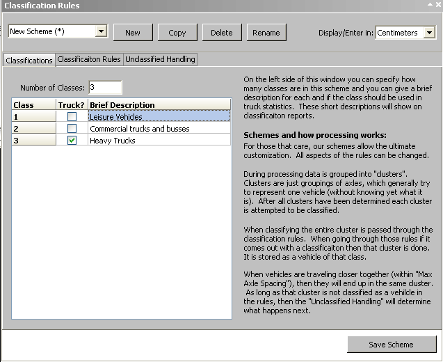
For this example, leisure vehicles would be motorcycles, cars, pickups, SUVs, etc. Commercial vehicles would be large vans, delivery trucks, buses, and motorhomes. Heavy trucks would be Dump Trucks and Tractor-Trailer Semis of all types. The Truck? checkbox is usually used to indicate trucks that are per-axle load restricted and regulated, so special statistics for these show up in the reports.
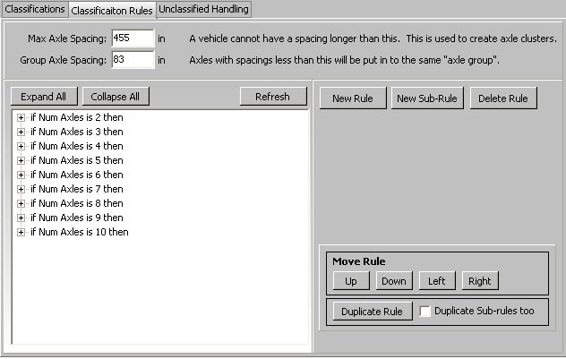
Now let us return to the Classification Rules tab. We first need to enter values for Max Axle Spacing and Group Axle Spacing and then click on the New Rule button. Let us Display/Enter in: Inches, so the panel would look something like this:
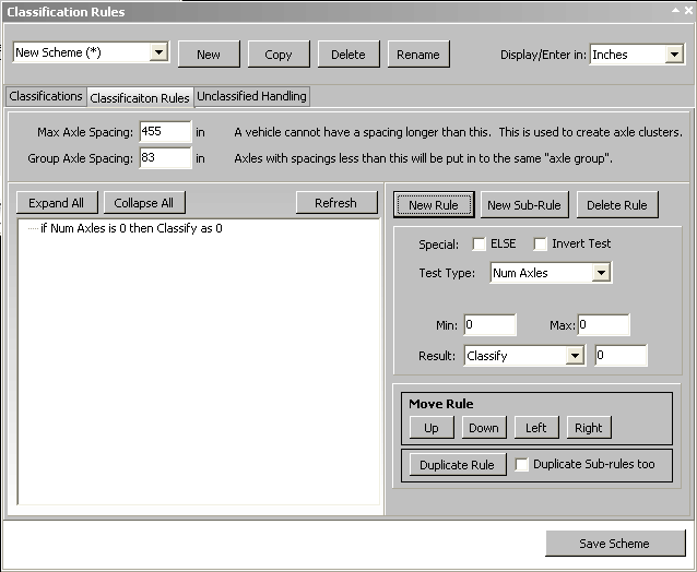
Note, we used the spacings from the default FHWA scheme to fill in the Max Axle and Group Axle fields for this example.
Now we need to fill in the first rule. First select the Test Type from the pulldown list.
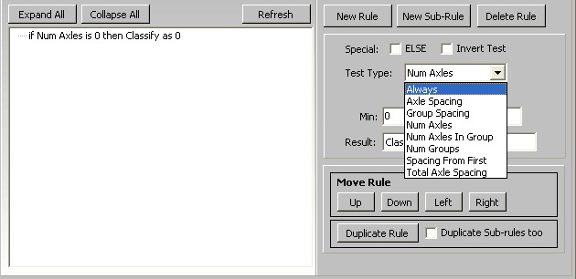
The list has the following rule test types available:
Always. This test type involves no parameters and will always be true. It may be placed at the end of a list of tests to force a result if all of the prior rule tests fail.
Axle Spacing. This test type is on axle spacing. If you choose this, you will need to enter the axle pair that the test is to be run on, and a minimum and maximum spacing to pass the rule. Note, that the number of axle pairs is always one less that the total number of axles in a cluster: Axle 1 to axle 2 spacing is axle pair 1, axle 2 to axle 3 spacing is axle pair 2, etc.
Group Spacing. This test type is on group spacing. It is similar to axle spacing, but only on the groups, rather than on individual axles (unless of course there is only one axle in the group). As discussed previously, groups are formed by axles that are equal to or closer together than the Group Axle Spacing parameter. The group spacing is considered to be from the last axle in the first group of a group pair to the first axle of the second group (in other words, the length of the gap between groups).
Num Axles. This test type is for the number of axles in the cluster.
Num Axles in a Group. This test type is on the number of axles in a particular group.
Num Groups. This test type is for the number of groups in the cluster.
Spacing from First. This test type is the spacing from the first axle to a specified axle.
Total Axle Spacing. This test type axle spacing from the first to the last axle in a cluster (roughly equivalent to total vehicle length).
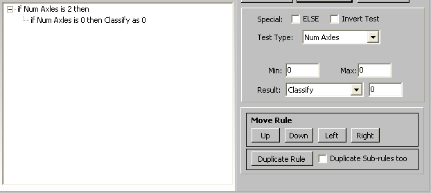
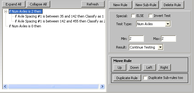
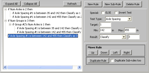
Let us set the first rule for all clusters with only two axles. So highlight the first (and only) rule and select the Num Axles for the test type. Next fill in 2 for the Min: field (note that Max will automatically fill with 2 also). Then select a result of a successful match:
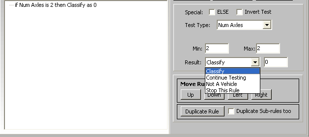
In this case, we need to do further testing to see what class the vehicle might be, so we will choose Continue Testing. The other options Not a Vehicle would only be chosen if all prior tests had failed and you did not want any subsequent testing to be run on the cluster data (in other words you wish to force re-clustering). Stop this Rule would be chosen if you did not want any further tests at this sub-rule level to be executed.
Since two axle vehicles could fall into more than one class (leisure vehicles, or commercial vehicles in our example), we need to do further testing, so we will need to add a New Sub-Rule, so we will click on the New Sub-Rule button.
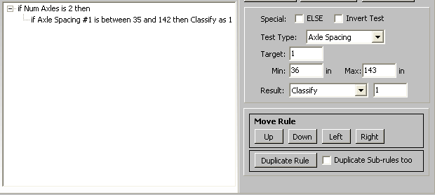
Let us say any vehicle with an axle spacing of 36 to 142 inches will be considered a class 1 vehicle (leisure vehicle), and vehicles with an axle spacing of 142 to 455 inches will be considered a class 2 vehicle (commercial truck or bus). So we set up this Sub-Rule by selecting Axle Spacing as the Test Type, a Target value of 1 for axle pair 1, a Min of 36 inches and a Max of 142 inches, a result of Classify as Class 1.
Now with our just created rule highlighted, click on the New Rule button which will give us a new rule at the same level as the highlighted rule.
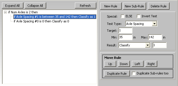
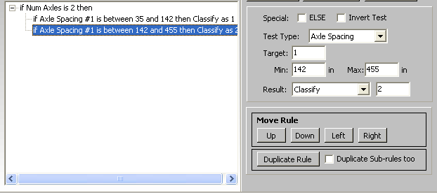
So now highlight the new sub-rule and fill in as Axle Spacing, Target 1, Min 142, Max 455, Result - Classify as class 2.
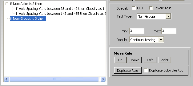
This finishes our first rule which is for 2 axle vehicles which classify as class 1 or class 2. However, class 1 and class 2 vehicles could also be towing trailers which need to be accounted for and may add one or more axles. For this classification scheme we assume that no class 1 or class 2 vehicle will have a dual axle on the rear, all multi-axle tandem axles will be on heavy trucks only (class 3 vehicles), but a trailer towed by a class 1 or class 2 vehicle could have a tandem axle arrangement. A way to set up a rule for this is to look for vehicles that have 3 groups (front axle, rear axle and trailer axle(s)), but only have axle pair 1 spacings of a class 1 or class 2 vehicle. Therefore, we highlight our first rule and click on the New Rule button to set up a new rule.
Highlight the new rule, select Test Type as Num Groups, set Min to 3 (and Max to 3) and the Result to Continue Testing.
Next click on the New Sub-Rule button. Then edit the parameters as: Test Type of Num Axles in Group, Target to 2 (second axle/group), Min to 1 (we only want the second group to be a single axle), and Result to Continue Testing. With this sub-rule still highlighted click on New Sub-Rule.
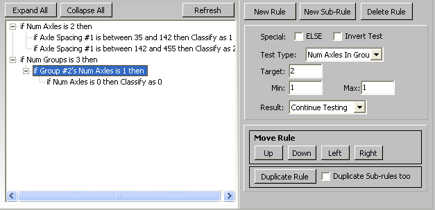
We now use the same axle spacing rules on the first axle pair as previously to differentiate the classes.
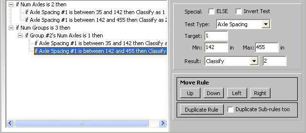
By now we have rules to catch all instances of class 1 and class 2 vehicles, but not every cluster that fails to fall into either of those two classes is necessarily a class 3 vehicle, so we need to make sure that the cluster is a Heavy Truck. We can determine this by checking the axle pair 1 axle spacings. Therefore, we will make a new and final rule (for this example). Highlight the last main rule and click on New Rule, then highlight the new rule, set Test Type to Axle Spacing, Target as 1, Min 142 and Max 455, Result - Classify as 3.
This is a quick study on how you would go about generating a new scheme. Actual schemes can be considerably more complicated to cover all possible variations of vehicle types. There is one more section, the "Unclassified Handling" which is discussed in detail below. Namely, if the cluster does not pass any of the rules then what happens to the cluster data must be defined. Once you are satisfied with your new Classification scheme, you may save it by clicking on the Save Scheme button at the bottom of the panel. If you have a data file open already, you will see the data overview re-calculate showing the new results immediately. Also note that as soon as you save the scheme, the rules box collapses all the rules automatically to keep things more readable. If you need to edit or review the details, you can expand each rule, or click on Expand All.
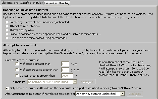
This tab allows you to dictate what to do when a cluster of axles has failed to be classified. This panel is organized into two areas; the upper area gives you five choices of what you may want to do, and the lower area contains the tests for your choice. We will discuss each of these options in more detail.
Do nothing. Leave cluster unclassifed/unhandled.
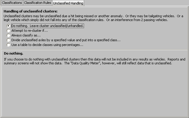
This option is pretty self-explanatory. The unclassified cluster of axle hits is just thrown away. This option might be most useful in very clean data where there are occasional bogus hits due to non-vehicular traffic such as bicycles, construction equipment, foot traffic, etc.
Attempt to re-cluster if...
This option is the recommended option for handling a cluster that fails to classify. The tests here dictate how the re-clustering is accomplished. By default re-clustering will occur if the unclassified cluster has more than 3 axles (or 3 axles if the Only allow a re-cluster if ALL.... checkbox is unchecked). However, you can modify this rule and others by activating various tests.
# of axles is greater than. This test if selected will allow you to limit re-clustering to clusters that have more than the specified axles.
# of axle groups is greater than. This test if selected will allow you to limit re-clustering to clusters that have more than the specified groups.
Cluster length is greater than. This test if selected will allow you to limit re-clustering to clusters that represent more than the specified total length (distance from first axle in the cluster to the last axle in the cluster).
As mentioned in the panel descriptive text, any one or all of these limiting tests can be selected. If multiple tests are specified, they are effectively OR'ed together. For instance in really heavy traffic, you may want to specify that the cluster length cause a re-clustering.
Only allow a re-cluster if ALL... This checkbox will only allow re-clustering if ALL of the axles in the cluster eventually get used in classifying vehicles. For light to medium traffic this is a good option, it maximizes accuracy. However, in heavy traffic, you may find that unchecking this box gives better results.
After attempting to re-cluster, if... This pull-down list gives you several options on what to do with the cluster if it fails to re-cluster. These are the same options that we have if we chose not to re-cluster in the first place.
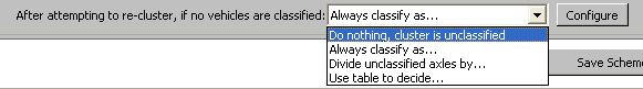
After you have selected what you want to happen to the failed re-clustering data, click on Configure to display and edit the test panel for that option (same as the test panels for those options discussed above and below this option, except for the appearance of a <<<Back button which allows you to return to this test panel after setting the tests). This insures that data that fails re-clustering still gets handled in a meaningful way.
Always classify as...
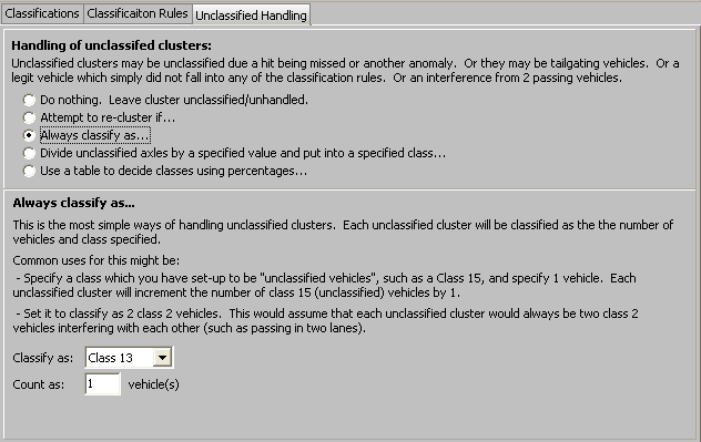
As stated in the panel description, this option would allow you to place the unclassified cluster (or partial cluster if this was the final result of the attempt to re-cluster) into a special class for unclassified vehicles. Alternatively, if the traffic is primarily cars and small pickups and SUVs, you could treat any unclassified cluster as 2 vehicles, such as 2 class to vehicles, assuming the cluster was probably due to interfering vehicles.
Divide unclassified axles by a specified value and put into a specified class...
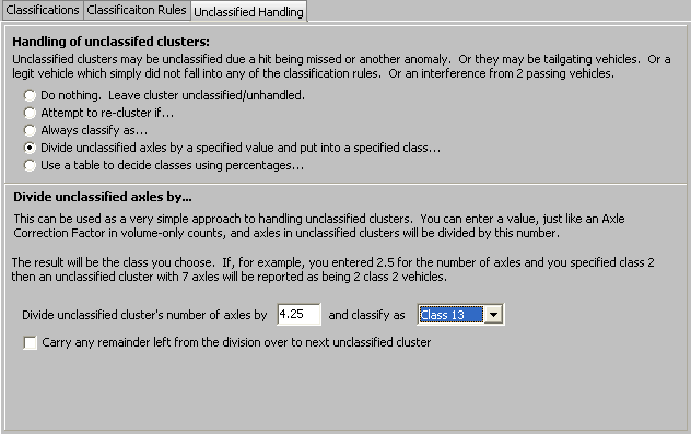
Again the description on the panel explains pretty clearly how this option works. This option is similar to the Always classify as... option, except, if you know the statistical makeup of the vehicles in the study, you could make a reasonable estimate of the makeup of the unclassified cluster in partial axle counts and reduce it to a single class.
Use a table to decide classes using percentages...
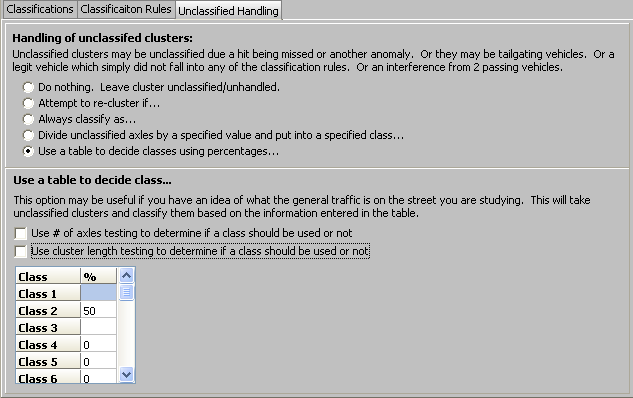
This option can be used to classify unclassified clusters effectively when you have statistical knowledge about the traffic make-up (the average the vehicle distribution by class). This would be most useful in very heavy congested studies when the normal methods are resulting in a significant number of incorrect classes or unclassified vehicles. It would not be appropriate in studies where you have no reasonable knowledge of the traffic make-up.
As shown, you can have unclassified vehicles be classed according to a distribution table. The "%" column indicates what percent of the unclassified clusters will be assigned to that class. The percentages in the "%" column must add up to 100%. For instance, if a cluster fails to classify, then this option will assign the cluster to a class based on the percentage of likelyhood it is a particular class. For instance, according to the above settings, if there were 100 unclassified clusters in the data file, 50 of them would be classed as class 2, etc.
In addition to just a simple percent distribution, you can also add tests for the number of axles, and/or the total cluster length (from first axle to last axle in the cluster), for each classification, to further refine correct distribution of the probabilities. If you wish to use either or both of these tests, just check the appropriate checkbox. When you do this additional columns will show up in the table to allow you to set minimum and maximum parameters for axle counts and total length. For example with both tests checked, the table will expand and would look something like this:
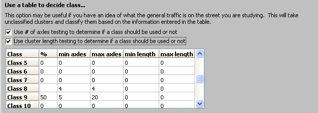
At the bottom of the Classification Rules panel is a Save Scheme button. When this button is clicked, any and all changes made to the highlighted scheme in the schemes list will be saved to that scheme. Note! If you modify one of the default schemes and save it, it will now show with a (*) symbol following it. Your modified version will now take precedence over the default scheme. If you should later delete or rename this scheme, the original default scheme will once again become active.